Spectrum Analyzer
Overview
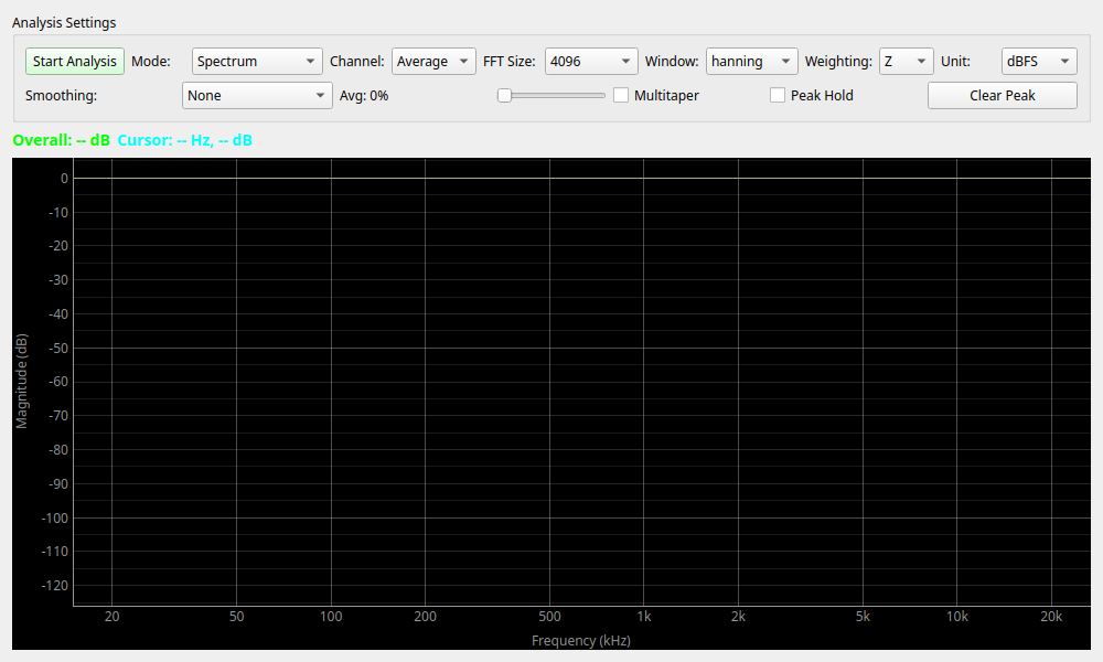
This tool analyzes and displays the frequency components of audio signals in real-time.
You can visually confirm the magnitude of each frequency band for sounds input via microphone or line-in.
In addition to general FFT (Fast Fourier Transformation) analysis, it also features advanced measurement functions such as PSD (Power Spectral Density) display useful for noise analysis, and weighting (A-weighting/C-weighting) that takes hearing sensitivity into account.
Operation
Starting and Stopping Measurement
- Start Analysis / Stop Analysis button: Toggles the measurement start and stop.
Reading the Graph
- Horizontal Axis (Frequency): Represents frequency (the pitch of the sound). Moving to the right indicates higher pitch. It is displayed on a logarithmic (Log) scale.
- Vertical Axis (Magnitude): Represents the size (strength) of the signal. Moving upwards indicates a stronger signal. The unit for the scale depends on the settings (Unit).
- Cursor: When you hover the mouse cursor over the graph, the exact frequency and level at that point are displayed in "Cursor: ..." at the top of the screen.
- Overall: Displays the total signal level (root mean square) across the entire frequency range.
Settings
Basic Settings (Analysis Settings)
-
Mode
- Spectrum: The most common mode. Displays the peak levels for each frequency. Suitable for measuring signal levels such as sine waves.
- PSD (Power Spectral Density): Displays the power spectral density. Use this when you want to evaluate the noise distribution uniformly. The unit is .
- Cross Spectrum: Displays the correlation components between the L and R channels (advanced setting).
-
Channel
- Left / Right: Displays only the specified channel.
- Average: Displays the average of the left and right channels.
- Dual: Displays both left and right channels simultaneously on the graph (Left=Green, Right=Red).
-
FFT Size (Frequency Resolution)
- Specifies the number of samples used for analysis.
- Higher values (e.g., 131072, 1M): Increases frequency resolution, making it easier to distinguish dense peaks, but the response speed over time becomes slower.
- Lower values (e.g., 1024, 4096): Decreases frequency resolution, but the response speed over time becomes faster, allowing it to easily follow fast-moving sounds.
- Usually, a value between
4096and16384is recommended for a good balance between resolution and response speed.
-
Window (Window Function)
- A process that smoothly tapers the edges of the sampled waveform to suppress errors (spectral leakage) caused by discontinuous cutoffs during FFT analysis.
- hanning: The most versatile and common window function. Choose this if you are unsure.
- rect (Rectangular): No window function is applied. Errors will be large for any signals other than transient signals or signals whose cycles match perfectly.
- Multitaper: When the Multitaper feature (described below) is turned ON, a dedicated window function is automatically applied.
-
Weighting
- Z: No weighting (flat). Use this when measuring physically accurate voltage or sound pressure.
- A: A-weighting. A filter that matches the sensitivity characteristics of the human ear (sensitive to mid-frequencies, less sensitive to low and high frequencies). This is the standard setting for measuring noise levels.
- C: C-weighting. Closer to flat than A-weighting, but it cuts out very low and very high frequencies that human ears cannot hear. It is often used to evaluate the sound pressure you "feel" with your body at loud venues like live houses.
-
Unit
- dBFS: A relative value with 0 dB as the digital full scale. It is the level relative to the input limit of the audio interface.
- dBV: Voltage level with 1 V as 0 dB (requires calibration settings).
- dB SPL: Sound pressure level (requires calibration settings such as microphone sensitivity correction. If uncalibrated, it automatically falls back to dBFS).
Advanced Controls
-
Smoothing
- Smooths out the jaggedness of the graph to make it easier to read.
- 1/3 Octave, etc., are common display formats used in audio analysis.
-
Avg (Averaging)
- Specifies the strength of the averaging process in the time direction.
- Moving the slider to the right makes the graph move more slowly, suppressing fluctuations in noise components for easier viewing.
-
Multitaper
- When turned ON, it uses multiple window functions to reduce the variance (scatter) of the spectrum estimation. This can result in smoother and more reliable results in noise analysis. When ON, the Window setting is disabled.
-
Peak Hold
- Continues to hold the maximum level from the past with a red dotted line.
- Convenient for checking loud sounds that occur only momentarily.
- Clear Peak button: Resets the held peak display.
-
RTA Mode
- Changes the graph display from a standard continuous line plot to a Real-Time Analyzer (RTA) bar graph format.
- When RTA Mode is enabled, the frequency spectrum is aggregated and visualized as discrete vertical bars according to the selected Smoothing resolution (e.g., 1/3 Octave). This provides a more traditional acoustic measurement view.
Usage Examples
Below are a few specific usage scenarios for the Spectrum Analyzer.
Basic Input Check
Basic usage to confirm that the microphone is picking up sound correctly.
- Press the Start Analysis button to begin measurement.
- Select
Spectrumfor Mode andAverageorLeftfor Channel. - Speak into the microphone or clap your hands.
- If the graph reacts and changes shape, the input is functioning normally.
- By turning ON Peak Hold and clapping, the frequency components of the momentary impact (the spectrum of the pulse sound) will remain as a red line, making it easier to observe.
Noise Floor Measurement
Checks the noise level (noise floor) when there is no sound. This is useful for improving the S/N ratio or finding power supply noise.
- Connect the input device (microphone or line input) and ensure no sound is being produced.
- Change Mode to
PSD. PSD is suitable for viewing the distribution of noise. - Increase the Avg (Averaging) slider to about
50%to90%. The jumpiness of the waveform will subside, and the average noise line will become visible. - If there is a sharp peak at a specific frequency (e.g., 50 Hz or 60 Hz), there may be power supply hum noise mixed in.
- Setting Smoothing to
1/3 Octavemakes it easier to grasp the overall noise trend (whether it's closer to white noise or pink noise, etc.).
Speaker Frequency Response
By playing a test signal (such as pink noise) and picking up the speaker's output with a microphone, you can perform a simple check of the frequency response.
- Prepare and play a Pink Noise source separately.
- Place a measurement microphone in front of the speaker.
- Set Mode to
Spectrumand FFT Size to around16384. - Set Avg to a high value (
90%or more). - Set Weighting to
Z(flat). - As the graph approaches flatness, the speaker's characteristic is flat. If the low or high frequencies are drooping, that is the limit of the speaker's reproduction range.
- This is not a rigorous measurement as it also picks up room reflections, but it is effective for knowing trends.
Automatic Peak Markers
Open Peaks: Off at the upper-right of the plot to configure markers. Existing analysis controls and Peak Hold work independently.
- Off is the default. No peak detection runs. Marker graphics are allocated only on first use, then reused.
- Display peaks detects maxima in the displayed trace after smoothing or pixel-envelope aggregation, or in the RTA bands. Envelope minima and maxima at the same frequency are combined before detection. Frequencies are display bin/band centers and can change when zooming or resizing.
- Raw-spectrum peaks detects FFT-bin maxima before display smoothing and envelope aggregation. It retains the selected analysis mode, channel, averaging, calibration and frequency weighting; it is not unprocessed audio. Raw markers can lie above a smoothed trace or RTA bar. No sub-bin interpolation or measurement-accuracy claim is implied.
The button identifies the selected source and level unit, including weighting
and /√Hz in PSD mode. Each marker gives frequency in Hz and level in that unit.
Dual mode labels identify Left or Right; spacing applies separately per channel.
- Local prominence, in dB, rejects peaks that do not rise sufficiently above their surrounding valleys. The neighborhood is at most 2049 source points centered on each peak; this bounds work on large FFTs. Broad peaks can therefore have lower local prominence than their height above the distant noise floor.
- Minimum spacing, in Hz, keeps the stronger peak when candidates in the same channel are too close. It is independent of the logarithmic axis scale.
- Noise floor is an absolute minimum peak level in the displayed unit, not an automatically estimated noise statistic. Changing units reinterprets this numeric threshold in the newly selected unit; review it in the settings dialog.
Defaults are 6 dB prominence, 100 Hz spacing and a −90 noise-floor threshold. Settings last for the lifetime of the widget. OK applies them to the next live frame; Cancel leaves them unchanged. Up to five strongest visible peaks across both channels are marked, with detection refreshed at most five times per second while conditions remain unchanged. Raw mode reduces this limit to roughly one update per second at the largest (4M) FFT, without changing spectrum refresh. Condition and viewport changes invalidate old markers. Labels that overlap or extend outside the plot are hidden; position symbols remain. Flat traces, endpoints and invalid values are not reported as peaks. Detection does not add work to the audio callback or retain frame history. Stopping retains the latest overlay; restarting or changing analysis settings clears it until the next live frame. Markers are display aids and are not included in exported spectrum data.