Response Viewer
Overview
The Response Viewer is an advanced visualization tool for analyzing linear and harmonic response characteristics (up to the 5th order) extracted by the Nonlinear Analyzer. It allows you to deeply evaluate the measured Hammerstein model's frequency response and simulate the system's output behavior (e.g., gain compression) at arbitrary frequencies and amplitudes.
Key Features and Operation
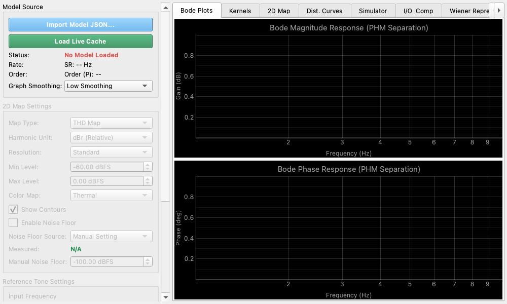
Model Source
- Load Live Cache: Directly loads the most recent model measured and extracted by the Nonlinear Analyzer.
- Import Model JSON...: Loads a previously saved Hammerstein model from a JSON file.
2D Map
- Map Type: Selects the type of map to display.
- THD Map: Map of Total Harmonic Distortion relative to the fundamental.
- Distortion Map (nth): Individual maps for the 2nd to 5th harmonic components.
- Harmonic Unit: Selects whether to display levels in relative (dBr) or absolute (dBFS) units.
- Resolution: Adjusts the calculation resolution of the map (Overview, Standard, Detail).
- Min/Max Level: Sets the display range for the input amplitude (Y-axis).
- Color Map: Changes the color palette of the map.
- Show Contours: Draws contour lines on the map.
- Enable Noise Floor: Factors in either the measured noise floor or a manually set noise floor into the plots.
Dist. Curves (Distortion Curves)
- Reference Tone Settings: Sets the "Input Frequency" and "Input Amplitude" as the reference point for evaluation.
- The upper plot displays the distortion characteristics across a frequency sweep at the reference amplitude, while the lower plot shows the distortion across an amplitude sweep at the reference frequency.
Simulator
- Simulates and displays the predicted output spectrum as a bar graph, assuming a pure sine wave is input at the set reference frequency and amplitude.
- A detailed list of the predicted amplitude and phase for each harmonic is also provided.
I/O & Comp (Input/Output & Compression)
- Input-Output Transfer Curve: Visualizes the transfer characteristics (ideal linear output vs actual output) at the reference frequency and estimates the system's 1dB compression point (P1dB).
- Gain Compression: Plots the deviation (compression error) from the ideal linear gain.
Wiener Settings
- Equivalent Gaussian RMS Level (σ): Configures the equivalent RMS level () in dBFS of an input Gaussian noise signal. By default, it is synchronized with the Reference Amplitude.
Wiener Representation
Converts the measured Hammerstein kernels into Wiener kernels () in both the frequency and time domains using Hermite orthogonalization relative to the input RMS level (). This allows you to evaluate the orthogonalized distortion profile at specific operational levels.
- Wiener Kernel Magnitude Response: Plots the gain frequency response of each Wiener kernel (dB vs Hz, logarithmic X-axis).
- Wiener Kernel Phase Response: Plots the phase frequency response of each Wiener kernel (deg vs Hz, logarithmic X-axis).
- Wiener Kernel Energy Fraction: Renders the time-domain energy fraction (%) of each Wiener kernel as a bar graph, visualizing the contribution of distortion energy for each order.